In a previous tip, we showed you how to set up a PivotTable using PowerPivot. You’re now going to learn how you can easily calculate Sales Tax/ VAT using the Measures feature in the PowerPivot tab. If you’re the business’s accountant, you may want to analyze the Sales Tax/ VAT that will be paid on the products you’ve sold. Luckily, the Measures feature in the PowerPivot tab enables you to create formulas in your PivotTable.
We’ll show you how in the steps below.
Applies To: Microsoft Excel 2010 and 2013
1. Open the example exercise workbook, where a PivotTable is set up.
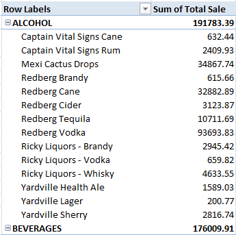
2. Select any cell within the PivotTable.
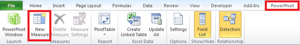
3. Select the PowerPivot tab and then New Measures under the Measures tab. Refer to the screenshot below.
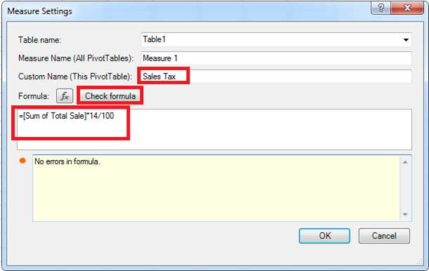
4. In the Measure settings screen:
a. Rename the custom name to Sales Tax.
b. Enter the formula: =[>Sum of Total Sale]*14/100
i. Press the left square bracket key.
ii. Select Sum of Total Sale from the drop down list.
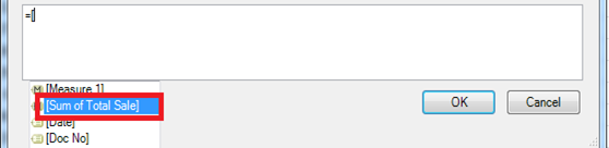
iii. Then enter *14/100
c. Click on Check formula, to ensure that the formula is correct.
5. Select OK.
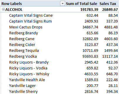
The PivotTable with a calculated field (Sales Tax) will be displayed. The percentage rate for Sales Tax will vary for each country—we used 14% for illustration purposes. Measures can also be used to create advanced functions on PowerPivot.