Last week we showed you how to install the PowerPivot add-on module in Microsoft Excel 2010 and 2013, and how you can use it to process immense volumes of data that cannot be efficiently handled by PivotTables. Today, we want to show you how to set up a PivotTable using PowerPivot to enable you to analyze large volumes of sales data efficiently. We will use a Product Sales by category report as our example.
You are welcome to download the workbook to practice this exercise.
Applies To: Microsoft Excel 2010 and 2013
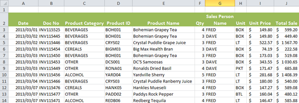
The data below will be used to create a PivotTable using PowerPivot.
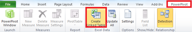
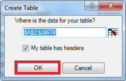
1. Select the PowerPivot tab, and Create Linked Table in the Excel Data group, and them select OK.
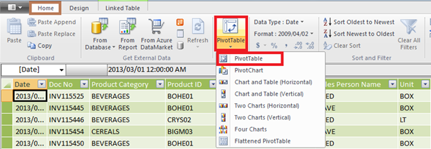
2. Select the Home tab and PivotTable.
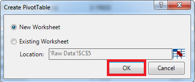
3. A Create PivotTable screen will pop up. To place the PivotTable on a new worksheet, select New Worksheet and OK.
4. Using the field list placed on the right hand side of the worksheet arrange the fields into the different areas of the PivotTable
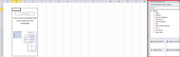
5. Place the fields as follows:
- Product Category, Product Name (Rows labels area)
- Total Sale (Values area)
- Sales Persons Name (Slicers Horizontal)
6. The PivotTable will be displayed.
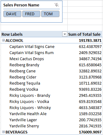
The PivotTable displays the Product Sales by category. Slicers, which are used to easily filter components are part of the PivotTable field list and are automatically added to the PivotTable. By clicking on a Sales Person, say Dave, you are able to filter on the transactions or sales made by Dave.
