Currently, there’s no function that will convert dates into quarters in Microsoft® Excel®. However, using the CHOOSE function, we can easily convert dates into quarters in Excel.
The CHOOSE function returns a value from a list of items based on a position number. For example, if we had a function =CHOOSE(3,”Apples”,”Bananas”,”Peaches”,”Pineapples”) the function would return “Peaches”, as that is the third item in the list supplied. If you replaced the 3 with a 2, then “Bananas” would be returned.
To achieve our objective, we are going to use the MONTH function together with the CHOOSE function to return a list of quarter numbers.
You are welcome to download the workbook to practice.
Applies To: Microsoft® Excel® 2010, 2013 and 2016.

The formula in cell D4 uses the MONTH number for the date in cell B4, and returns the quarter that corresponds to that number. As August is the 8th month, Excel will return the 8th item from the list supplied, and will return a 3 for the quarter. When calculated, August does fall into the 3rd quarter of the year.
By adjusting the order of your list, you can easily manipulate which quarter a month will fall into. If, for example, your financial year starts on the 1st June 2016 and you need to know which quarter a given date will fall into, simply adjust your list to correlate with your financial year start month.
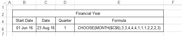
As June is the 6th calendar month, you would need to start entering quarter 1 at the 6th position and continue from there.
By using quarters, you are able to analyze data quickly and easily. There is no need to create Pivot Tables in this case as quarters can easily be created by using a formula.
