Slicers are used for filtering data and gives you a better understanding of your information. By using slicers you can quickly drill down on a PivotTable. Slicers also indicate the current filtering state, which makes it easy to understand what exactly is shown in a filtered PivotTable report.
You can save time by linking slicers to multiple PivotCharts, instead of inserting a separate slicer for each PivotChart.
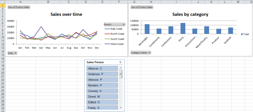
Any changes that you make to a shared slicer is reflected immediately in all PivotCharts linked to the slicer. In our example, we are going to share the sales person’s slicer by linking it to the sales by branch and sales over time PivotCharts.
Note: Please download the workbook to practice this exercise
Applies To: Microsoft Excel 2010 and 2013
1. Select one of the PivotCharts.
2. Select the Analyze tab.

3. Select Insert slicer.
4. From the list, select sales person. Then select OK.
5. Right click on the slicer. Then select PivotTable
6. Tick all the check boxes and select OK.
7. To analyze the performance of a sales person, select the name from the slicer.
8. To make multiple selection: press the CTRL key and select the names from the slicer list.
9. To clear the filter: click in the top right corner of the slicer.
By linking one slicer to multiple PivotCharts, you make your process more efficient and this helps save time, because the slicer will not be duplicated. You can also easily select the data you want to be filtered and have an overall view of the operations of the business. Ultimately this will help you make better business decisions.
