When extracting data from a database, dates don’t always show up in the format you want them to. That’s why it’s helpful to know how to use the Text to Columns option to convert dates into a format that can be used to easily analyze or work with data.
As an accountant, you may want to analyze data with Pivot Tables, and group by months, years or quarters. That can only be achieved if the dates are correctly formatted.
Follow the example below as we explain how this can be done.
You are welcome to download the workbook to practice.
Applies To: Microsoft® Excel® 2013 and 2016.
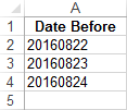
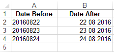
1. Highlight the data range A2 to A4.
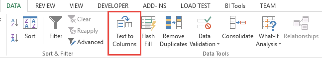
2. To convert the above into usable data, select the dates, then select the Data tab, and then Text to Columns.
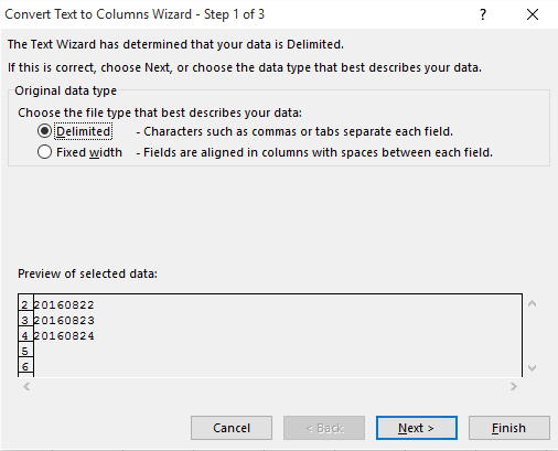
3. The Convert Text to Columns Wizard is now visible.
4. Select “Next” twice to get to Step 3. In Step 3, select Date and YMD.
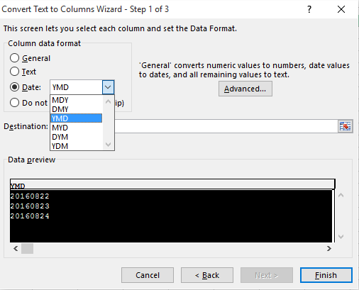
5. To override the selected dates, click Finish, or alternatively, enter a Destination cell.
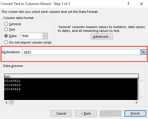
If you have entered a destination, the newly converted dates will be entered starting at the specified cell.
Now that you know how to convert dates into the correct format, you will be able to easily analyze the data with functions of Excel like Pivot Tables. Manipulating dates with formulas will also be simplified, thus saving you time.
