A dynamic drop down list in Microsoft® Excel® is a convenient way of selecting data without making changes to the source. Let’s say you have a list where you are likely to add or remove values, a dynamic drop down would be the best option to select data. With a dynamic drop down list, when you delete or add months the list changes to accommodate that action, whereas a normal list does not.
We have written tips on how to create a static and dynamic drop down list using and the Table option. However, in this tip we show you how to create a dynamic drop down list by using Data Validation, OFFSET and COUNTA functions.
We learnt in our previous tip that the OFFSET function is used for creating dynamic data ranges. The COUNTA function counts the number of cells that are not empty in a range. Data Validation is used for restricting what type of data should or can be entered into a range.
Note: Download the workbook to practice
Applies To: Microsoft Excel 2010 and 2013
1. We start by creating a defined name
a. Select the Formulas Tab, then Define
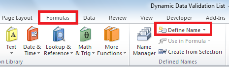
b. Enter Months under the Name text box
c. Enter =OFFSET(List!$B$2,0,0,COUNTA(List!$B:$B),1) under the Refers to text box

Here is a breakdown of what the formula represents:
- $B$2 refers to the reference or starting point
- The number of rows you want to move from the starting point is 0
- The number of columns you want to move from the starting point is 0
- The height in number of rows is COUNTA(List!$B:$B)
COUNTA(List!$B:$B) ,counts the number of values that are not empty in column B. When you add a value to the range, the number of values that are not empty will increase. The number of values that are not empty will decrease when you delete a value from the range. Therefore the named range expands when you add a value and contracts when you delete a value.
- The width in number of columns is 1
d. Select OK
2. To create a data validation list:
a. Select the Dashboard worksheet, then select cell N2
b. Select Data Validation under the Data Tab
c. Select List under Allow
d. Place the cursor in the Source text box and press F3. Then select Months
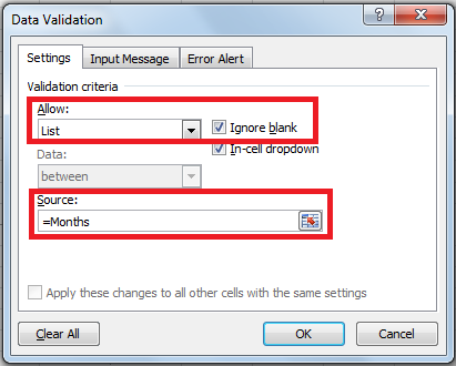
e. Select OK.
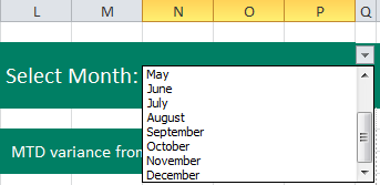
3. Select the drop down list in cell Q2.There are only six months in the list

4. Select the List worksheet and increase the number of months to December(12)
5. Select the drop down list in cell Q2 in the dashboard worksheet. The number of months has increased to 12
Based on the above example, the number of months in the data validation list will decrease if you delete some values from the range B2 to B13 on the list worksheet. Therefore a data validation list has been created, allowing flexibility when selecting data.
