Last week we shared a budget template to help you manage your finances. This week we want to show you how to use Icon Sets to see, at a glance, whether you’re over, below or on budget. In the template, you will see that we’ve used Icon Sets to illustrate the difference or variance between the projected cost and actual cost of an item. But, we haven’t applied them in the food category – we’ve left that for you to try out!
Applies To: Microsoft® Excel® 2010 and 2013
- Download the budget template workbook.
- Select the monthly budget worksheet.
- Select the data range E40:E42 – that’s the food category we left for you.
- Select the Home tab, then Conditional Formatting under the styles group.

- Select Icon Sets.
- Select three arrows.

- Click Conditional Formatting and select Manage Rules.

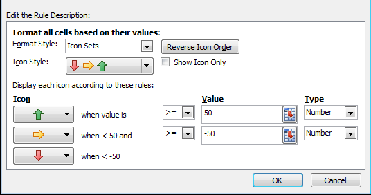
- Select Edit Rule. Here we will specify the criteria for assigning the icon sets is as follows:
a. Green: if the difference between the projected and actual costs is greater than $50. This means that the amount spent is $50 (and more) less than what was budgeted.
b. Red: if difference between the projected and actual costs is less than -$50. This means that the amount spent is $50 (and more) over budget.
c. Yellow: if difference between the projected and actual costs is between $50 and -$50. This means that the amount spent was pretty much on budget.

- Enter as below:
- For the green arrow, enter 50 under value and change the type to number.
- For the yellow arrow, enter -50 under value and change the type to number.
- Select OK.
- Select OK.

You can see that actual amount spent on ‘groceries’ is less than -50 (in other words, we went more than $50 over budget), for ‘dining out’ the difference was more than 50 (in other words we went more than $50 under budget), and for ‘other’ the difference was between -$50 and $50.
