In this tip, we want to take this opportunity to address a very important issue faced by many people that use Microsoft® Excel®. Sometimes when working with PivotTables, the Count function is set as the default instead of the Sum function. This can be frustrating as you then have to set each column value to Sum. Here’s how to solve this issue.
The problem is caused by having blank cells in the PivotTable source data, and as a result, the values default to count. In order to rectify the problem, you have to replace the blank cells with zero values. Follow the instructions below to see how:
You are welcome to download the workbook to practice this exercise.
Applies To: Microsoft Excel 2010, 2013
1. To replace the blank cells with zero values in the example workbook.
a. Click on one of the values in the source worksheet.
b. Press F5
c. Click Special.

d. Select Blanks and then Select OK.

e. Enter 0 in one of the blank cells.
f. Press CTRL + Enter.

2. To create a Pivot Table with the Sum as the default.
a. Select any cell within the source worksheet.
b. Click on the Insert tab.

c. Select Pivot Table.
d. Click OK.
e. Move the Product Name field to the rows area.
f. Move the Product Sales field to the values area.
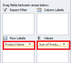

A PivotTable with the Sum function as the default will be created. However, if a PivotTable was set up with blank cells in the source data, the default for Products Sales would have been count instead of Sum.
