In our last tip, you were introduced to the new financial ratio reports provided through the Report Utility, which you can use to perform a health check of your business. If you didn’t catch it, or would like to brush up on it, you can find it here.
Although the reports are comprehensive, they don’t have every ratio that’s out there. There may be a few that you would like to add, and provided the source information is included, you can do so. In this tip, I’m going to show you how.
Working with Sage 300 Intelligence Reporting as an example, I’m going to add Effective Tax Rate to mine. Take note that this is the same example covered in webcast series included with the first tip. If you’d like to take a look at it, you can find the different videos here.
The new health check reports are available for the following products:
- Pastel Partner version 14 & 17
- Pastel Evolution version 7.0
- Sage 100
- Sage 300
To add the new financial ratio, work through the below steps. Take note that depending on your accounting product / business solution, the sheet names referred to here may differ slightly to yours.
1. Run out a copy of your report from the Report Manager.
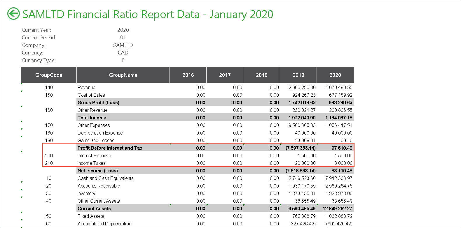
2. Once you have decided what ratio you want to add, check to see if you have the balances for it. You can do this by looking at the Financial Data worksheet. For Effective Tax Rate, I need Profit before Interest and Tax, Interest Expense and Income Taxes, and you can see that they are there.
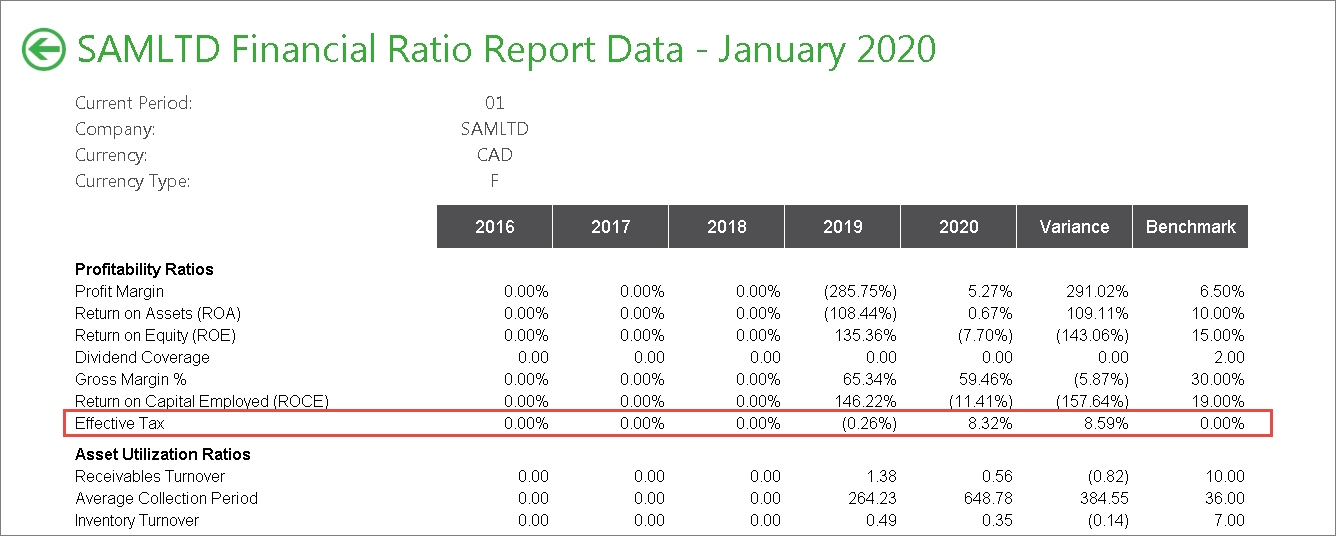
3. Now add the financial ratio to the Ratio Trend sheet.
- Insert a new row under the correct category and enter a description for it.
- In the first year column, add the calculation for it using the values from the Financial Data worksheet. In my case, Effective Tax Rate is calculated as:
Income Taxes / (Profit before Interest & Tax – Interest Expense) - Remember to use the correct referencing in the formula. You can then use Excel’s autofill functionality to drag it across to populate the other years. You can also drag down the variance and benchmark formulas and ensure the correct cell formatting.
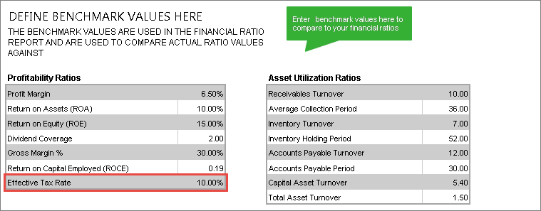
4. Next, add a new benchmark for the ratio in the Financial Report Settings sheet, giving it the value you want, and make sure it ties up with the formula in the Ratio Trend sheet. I’ve added mine at the bottom of my Profitability Ratios group.
5. Then, update the Financial Ratio Report sheet with the new information. This is a simple case of adding a new row for it, entering a description and copying the existing formulas down. Take note that your description will need to match the one used in the Ratio Trend sheet, as lookups to the values in that sheet are done.
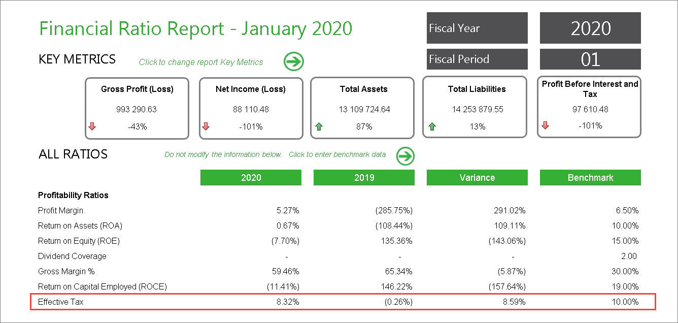
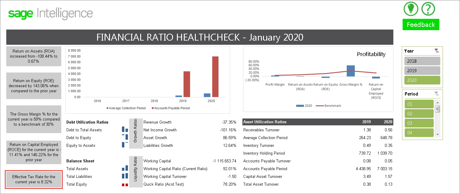
6. Lastly, you can update your dashboard to include the ratio. Depending on the one you’ve added, there may be different ways to do this. I’ve combined some text and a value reference for mine and included it with the descriptions on the left of my worksheet.
Once you’re finished, remember to save your changes using Save Excel Template in the Report Manager. You can see that with a little work, it’s easy to update your report, leveraging the information already contained in it, to suite your needs.
