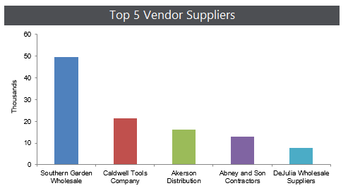
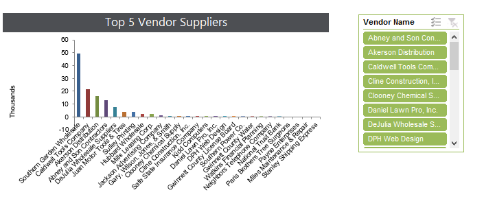
Charts are used for creating a graphical presentation of the data. A common practice when creating charts is to create them off of a filtered Pivot Table, usually a Top 5 or a Top 10 Pivot Table. Slicers can then be added to interactively filter the data in the chart.
When filtering data with the slicer, the filtered data on the chart can be reset. That is why in this tip, we explain how to prevent slicers from ruining top 10 charts.
Applies To: Microsoft® Excel® 2010, 2013 and 2016.
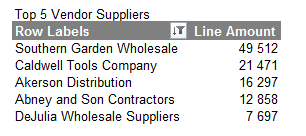
The Pivot Chart was created from the Pivot Table below.
A slicer was then added to the Pivot Table.
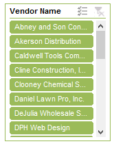
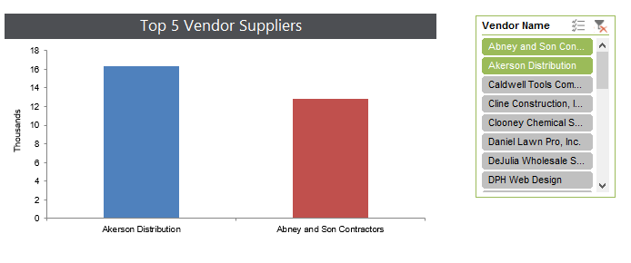
If you use the slicer to filter the data below, it appears to work correctly.

However, when you clear your selection by clicking the filter icon on the top right side of the slicer as seen below, then the filtering is lost.
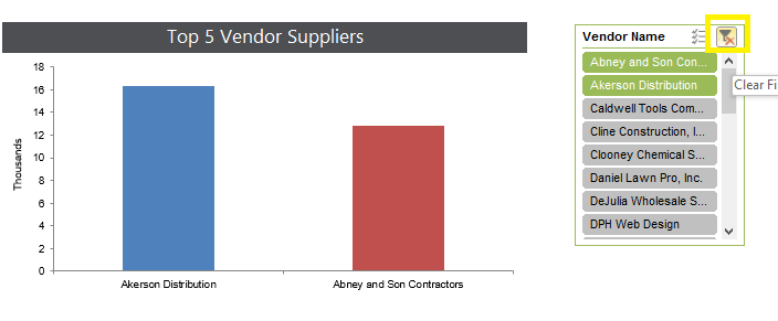
When you clear the slicer selection, Microsoft Excel clears the Pivot Table “Top 5” filter, including any other filters applied on the Pivot Table.
This causes the chart to reflect the raw, unfiltered data now appearing on the Pivot Table.
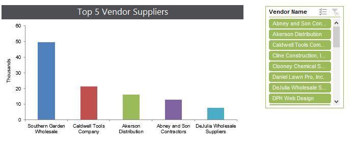
To prevent this from happening, ensure that, under your Pivot Table Options > Total & Filters Tab, the “Allow multiple filters per field” checkbox is ticked. To activate this option, right click on the Pivot Table, then select Pivot Table options.
Thereafter, filter your Pivot Table as required. The slicers will no longer get rid of your Pivot Table filters.
Slicers can then be cleared without clearing Pivot Table filters.
This is an essential tip when creating Dashboards that contain many filtered charts and slicers.
