As an accountant, you can easily categorize debtors balances by using the conditional formatting – icon sets option. Icon sets creates a visual effect in your data and helps you to see how the value of a cell compares to other cells. In the example below we categorize the debtors balances as follows: red icon for values greater than or equal to 20,000, yellow icon for values between 10,000 and 20,000 and green icon for values less than 20,000.
You are welcome to download the workbook to practice.
Applies To: Microsoft® Excel® 2010, 2013 and 2016.
- Select the data range C2:C24.
- On the Home tab, in the Styles group, select Conditional Formatting.
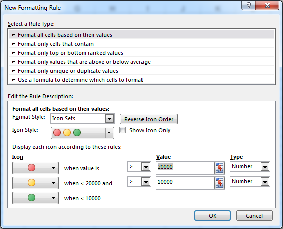
- Select Icon Sets, then more rules. Then select Reverse Icon Order.
- Change the Type from Percent to Number for both the red and yellow icons.
- Enter 20000 as the value for the red icon and enter 10000 as the value for the yellow icon. Then select OK.
Analyzing debtors balances will be done quickly and efficiently, which will result in to greater time saving. It also ensures accuracy in your data analysis. Inadvertently this will leads to increased productivity as less time will be spent correcting mistakes caused by allocating the wrong value to your customers.
