The PivotTable grouping option in Microsoft® Excel® allows you to see summaries of data by grouping it together so that less detail is shown. Grouping can be done automatically on date fields and the data summarised by days, months, quarters or years. However, you can also create your own custom groups. For instance, you can group your expenses by reporting categories, which is what we’ll demonstrate in this tip.
Note: Download the workbook to practice this exercise
Applies To: Microsoft Excel 2007, 2010 and 2013
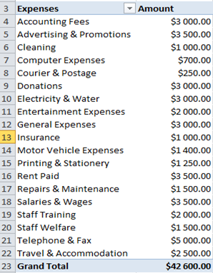
The example PivotTable has been populated with expenses and amounts.
To create the grouping for Admin expenses:
- Select all the expenses related to admin.
- Right click on one of the selected expenses.
- Select Group.
- Select the cell in the PivotTable now named Group 1 and rename it to Admin in the formula bar.
- Repeat step 2 for all subsequent grouping levels to be created.
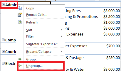
- To remove the grouping, right click on the group name and select Ungroup.
The PivotTable will thus be set up with the different grouping levels summarising the data.


