Do you have a workbook that could do with some neatening up? Being able to hide rows and columns in a report that contains data you don’t need to view is a great way to do this. An example of a report like this is a financial statement, which has account level detail and monthly columns with zero balances that don’t need to be shown.
It’s also a great idea to hide the rows and columns you don’t need to see automatically. This can be done using Macros. Following on from a previous tip; How to hide zero rows using Excel functionality, we have tweaked the Macros to make use of Named Ranges. Now, at the click of a button, all the rows and columns in your layout will update to reflect all accounts which have amounts against them—hiding those which don’t.
To ensure the workbook is completely up to date, the following procedures are run:
- Unhide all rows
- Hide zero rows
- Unhide all columns
- Hide zero columns
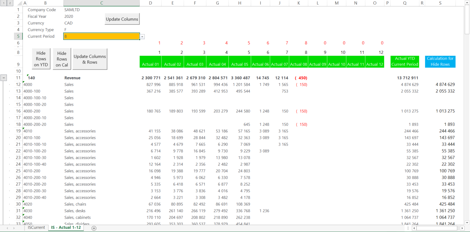
The below image shows an example of a workbook where rows and columns have not been hidden:
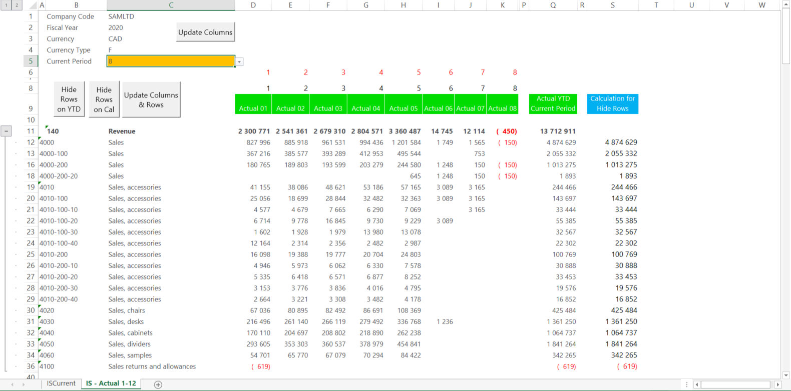
And the following shows the result after the Macros have been applied:
If this tip is what you’ve been looking for and you would like to better get to grips with it, take a look at the following webcast that will guide you through the steps:
The X-Factor Report Writers Series, Part 8: Final touches to your layout with Macros
The webcast also makes use of the following supporting documents which you can download here:
FRD Hide Zero Rows – Static values (Excel)
Neatening your workbook makes it easier for you to analyze your data, and saves you time in finding the information you need to make that business decision.
