In order to effectively analyze data, custom number formatting can be applied to your Microsoft Excel spreadsheet. Custom number formatting is used to easily identify values based on a set criteria. In a large Excel spreadsheet, you can easily highlight all negative or positive values by using custom number formatting.
In this example, we are going to display all negative values in a different colour.
You are welcome to download the workbook to practice.
Applies to: Microsoft Excel 2010, 2013 and 2016.
1. Select the range of cells which need to be formatted. For this exercise, we’ll use cells B1:B8 in the workbook.
2. Hold down the Ctrl and 1 keys simultaneously or right click, and select the Format Cells
3. Click on the Custom option under the Category section.
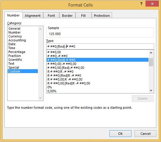
4. Select the # ##0; [Red] – # ###0 option from the Type list . The two parts are separated with a semicolon (;) to control positive and negative numbers only. Values to the left of the semicolon represent positive values and values which are to the right of the semicolon, represent negative values.
5. To remove the negative sign from the value displayed, the number format code must be adjusted by removing the sign from the format code as follows
With “– “
# ##0; [Red] – # ###0
Without “– “
# ##0; [Red] # ###0
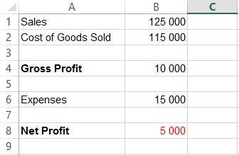
All negatives values are highlighted in red, making it easy to work with figures that have variances. This will save you time manually selecting all the negatives values, and will therefore increase your productivity.
