Manipulating data with missing labels can pose a challenge. Copying and pasting data can be time consuming and tiresome. That is why, in this tip, we show you how to quickly restore data labels using a simple formula.
If you find value in this tip, why not sign up for our Excel Tips and Tricks mailer, and get insightful tips delivered straight to your inbox on a weekly basis!
Below, we explain how that can be done.
You are welcome to download the workbook to practice.
Applies To: Microsoft® Excel® for Windows 2010, 2013, 2016
If you want to fill the blank cells of a column with the content above it:
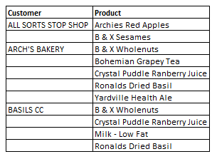
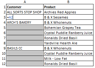
The starting point:
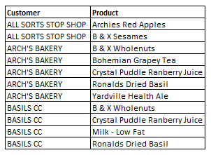
The goal:
The steps to get from start to the goal as follows:
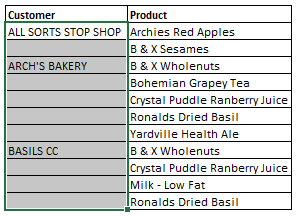
1. In Excel Highlight the column content you wish to fill, in this example, it would be the Customer column:
2. Click on the Home tab in Excel.
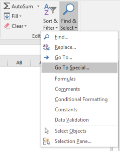
3. Click on Find & Select at the right edge of the Home tab.
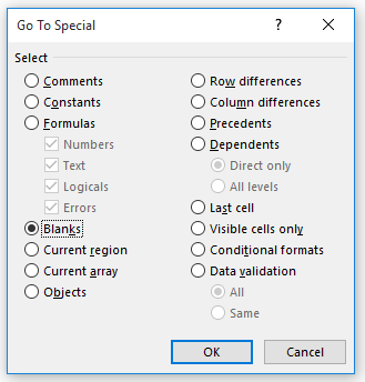
4. Select Go To Special:
5. Select Blanks and click OK, this will highlight the blank cells:
6. Holding down the Ctrl key, click the first cell under ALL SORTS STOP SHOP (i.e. A3), release the Ctrl key and type the formula =A2:
7. Holding down the Ctrl key, press Enter. This fills the blank cells with the relevant information:
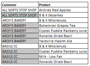
By filling in missing data, you are able to manipulate the data more easily. For example, you could unmerge cells, fill data, and apply a filter, and the data would not bring back blank cells.
