Accountants, bookkeepers and financial analysts alike will tell you one of the most sought after capabilities of a well-tuned accounting package is time efficiency. No one wants to spend unnecessary time having to enter monotonous data. This is where a well-specified reference sheet in your Sage Intelligence reports can be of immense help.
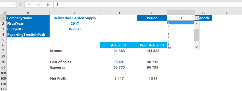
Take the following basic Financial Report Designer financial statement giving my Net Profit for the current and prior periods as an example.

This layout has been designed to make changing the period data easy, by changing the period number in cells D5 and E5. The same can be done for the year and budget code in cells C2 and C3. Although this works fine by just typing in the information, you can save time by being able to select the values from a drop down list. What would also be useful is if the corresponding month name could be shown along with the period values. This is particularly useful when dealing with a fiscal calendar that doesn’t follow the calendar year, i.e. does not run from January to December. The answer to this is to use a reference sheet.
To create one do the following:
- Make a copy of your report, rename it and run it out (in this case the Financial Report Designer)
- Add a new sheet to the workbook and rename it to something like “Reference Sheet”
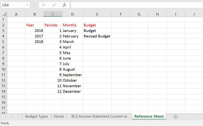
- Enter column headings for the lists and lookups you want to use
- Enter the data for your columns. In my case I’ve added data for my years, periods, months and budgets
You can now make use of the information in your layouts. The first thing I’m going to do is create a drop down for my periods:
- Select the cell where you want the list to appear. For me this is cell F1
- From the Excel ribbon, click on Data and then Data validation
- In the Data Validation dialogue, select List from the Allow field. Also make sure that In-cell dropdown is checked
- Then click in the Source field, select your reference sheet tab and choose the cells that contain your periods

- Click OK. You have now created your first drop down for your periods
- The financial formulas in the layout still need to reference the value selected in the drop down. The easiest way to do this is to reference the drop down’s cell in the existing period cells, in my case, D5 and E5. This can be done by entering the formula “=F1” into the cells.
Now by selecting a different period value from the drop down, the period values above the columns change as well and the data in the layout updates accordingly.
You can also now use your reference sheet to create a lookup that gives the month name for the period select from the drop down. In my case this will appear in cell H1. To so this:
- Select the cell where you want the month name to appear (H1 in my case)
- Use a lookup formula to return the month name in the reference sheet based on the value selected from the drop down. For me this is “=LOOKUP(F1,’Reference Sheet’!C3:D14)” – this is telling Excel to lookup the value in cell F1 in the periods column in the reference sheet and return the adjacent month name from the months column
You will see that when you change the period in the period drop down, the month name updates accordingly.

You can now look at creating drop downs for your fiscal years and budgets in the same way as the period drop down, and once finished will have created a more dynamic and efficient layout. Finally, hide the reference sheet. You may also want to hide the row above your column headings containing the period values to make your layout look neater. Then save your template back to your report in the Report Manager using Save Excel Template. The next time you run it out, the functionality you have added will be there and you can easily make your selections.
